
Navigating Uncertainty: Using Real Options to Improve Strategic Decision-Making
Part 4 of the "Navigating a Path to Success in the Age of AI" series


TL;DR
The rise of generative AI and other Collaborative Intelligence technologies has companies scrambling to understand and respond effectively to the prospective impacts on their competitive positions, business models, business processes, products and services, skills mix, etc. In addition, regulatory bodies and internal risk management organizations are scrambling to keep up.
The current business environment is tailor-made for Real Options. Real Options Valuation (ROV) is superior to traditional valuation approaches as a decision-support tool and a means for measuring and managing uncertainty and risk.
Companies would improve their chances of responding effectively to the many changes being wrought by generative AI by using ROV to support strategic decision-making.
A “strong form” of real options is used to value such things as mineral rights, oil leases, and patents. Strong Form applications have two things in common:
there is an underlying asset (e.g., gold, oil, prescription drug) that trades in public markets and
one company holds the exclusive right to exercise the option (mine, drill, launch).
This article focuses on the “weak form” of real options. Weak Form applications have three things in common:
there is a high degree of uncertainty about the future value of a specific investment,
decision-makers have the flexibility to do such things as delay investments or abandon previous investments,
the options are non-exclusive, meaning that other companies have similar investment options (e.g., entering an emerging market).
As 2024 begins, company executives face a complex and volatile business environment rife with uncertainties. Traditional valuation models (e.g., Net Present Value [NPV], Internal Rate of Return [IRR]) are not designed to support decision-making under uncertainty, potentially resulting in poor strategic decisions, misallocation of capital and other resources, reduced strategic agility, and the destruction of shareholder value.
Fortunately, an alternative valuation approach exists: Real Options. Real Option Valuation (ROV) addresses the many shortcomings of traditional approaches when making strategic decisions under uncertainty.
Rather than diving into real options immediately, I will demonstrate why they are necessary using a step-by-step approach.
Traditional Valuation: Net Present Value (NPV)
NPV is a method of calculating the Present Value (the value on the day the decision is made) of a series of future cash flows related to a specific investment. Since cash earned in the future is less valuable than cash earned today (this principle is known as the “time value of money”), future cash flows must be discounted at a specific rate.
NPV is calculated by subtracting the present value of all cash outflows (capital investments, operating costs, etc.) associated with the initiative from the present value of all cash inflows (revenues, etc.). If NPV is positive, decision-makers should invest.
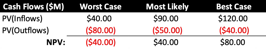
For example, if the Present Value (PV) of all cash inflows is $90M and the PV of all cash outflows is $50M, then NPV = PV(Inflows) - PV(Outflows) = $90M - $50M = $40M, and the investment should be made.
Although the valuation models that support real-world investment decision-making are much more complicated, the mechanism is the same.
Problem #1: Loss of Information Regarding Uncertainty
All valuation methods deal with future cash flows, so their values must be uncertain. No one can accurately predict the future, especially strategic investments with forecast horizons of 5+ years.
The problem with most spreadsheet-based valuation models (those that do not use any add-ins to support scenarios or more sophisticated approaches) is that the people populating the valuation model can enter only one specific value in each cell. Thus, pessimists may think the PV of future inflows will be $40M, and optimists may think they will be $120M. As a compromise, all agree to enter $90M (a slight positive bias from the midpoint resulting from the collective desire to “make the project look good”).
As soon as this happens, all information regarding the range of prospective outcomes is lost. Decision-makers, who usually do not participate in building the valuation model, have no idea what the range of possible outcomes could be.
This problem is exacerbated with every value entered in every spreadsheet cell. (You may think the inaccuracies cancel out when there are thousands of cells. They don’t.) Complicated spreadsheets with thousands of cells give decision-makers a false sense of security. They often mistake complexity for accuracy when, in fact, the opposite is true.
Table 1 depicts the example described above, expanded to include the uncertainty regarding outflows. (Table 1 mimics a situation in which modelers build three scenarios: best case, worst case, and most likely case).
This approach provides a marginal improvement, but in practice, with large, complex models, its value is limited because:
complex models make it difficult to detect biases (much easier in this example) and
each scenario provides only a single value, hiding the true range of outcomes and, in most cases, overstating the expected or most likely value.
Calculating and Depicting the Effects of Uncertainties and Biases
Calculating and depicting a range of outcomes rather than a single value requires either a third-party add-in for the spreadsheet software or a different modeling engine. Either must support the entry of probability distributions rather than discrete values and the ability to execute Monte Carlo Simulations.
Monte Carlo Simulations create thousands of scenarios rather than a few. In each scenario, random numbers are drawn from each probability distribution specified and used to calculate all other values in the model. All the results, taken together, create their own distribution of outcomes, enabling decision-makers to understand better how all the uncertainties combine to affect the value of the prospective investment.
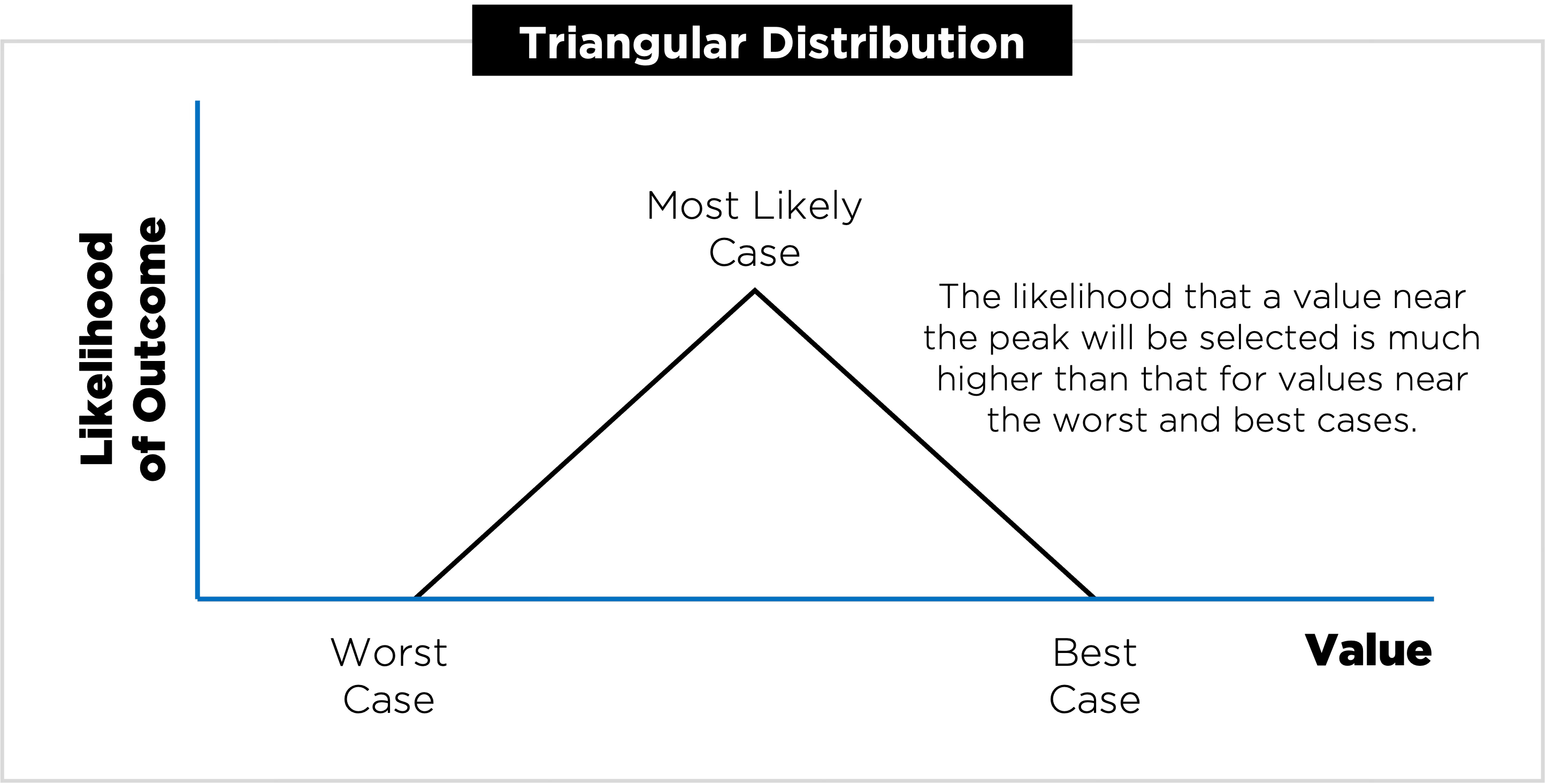
I used Python to model the situation in Table 1. I used a Triangular Distribution (Figure 1) to represent the best, worst, and most likely outcomes shown. However, I made one adjustment to eliminate the bias introduced in the original model. I used a Most Likely Case value of $40M for Inflows and -$60M for Outflows. (Absent a rational basis or expert judgment for skewing the most likely case toward the best- or worst-case value, the midpoint between the two extremes should be used. In the case above, the values were skewed for political reasons.)
I ran 10,000 simulations to calculate the NPV of this prospective investment, resulting in the outputs depicted in Figure 2.
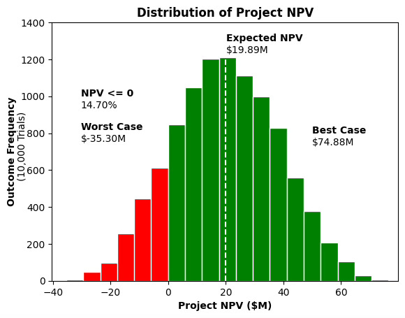
The best- and worst-case values are near those specified in Table 1, but eliminating the biases reduced the value of the most likely outcome (the Expected NPV value represented by the dashed white line) by 50.3% ($40M vs $19.89M). This is still a valuable investment, but much less valuable than previously estimated. Would decision-makers still approve this investment when other prospective investments are competing for the same limited investment resources?
The previous analysis showed a worst-case value, but the more pertinent question is, “What is the probability that this investment will lose money?” The previous analysis is silent on this question. Simulation results estimate a 14.7% chance the investment will not create any value (NPV = $0) or will destroy value (NPV < $0).
The previous analysis is also silent on the related question, “What is the probability that this investment will at least break even or create some value?” Simulation results estimate an 85.3% chance of breaking even or creating value with this investment.
In this simple case, using the previous analysis or this more sophisticated analysis would probably result in the same decision. In real-world cases, seeing simulation outputs often results in different decisions than those made using models that hide uncertainty and biases, resulting in better investment decisions and increased Return on Invested Capital (ROIC).
Problem 2: Inability to Accurately Model and Value Managerial Flexibility
When facing uncertainty, company leaders can defer investment decisions until the uncertainty is reduced (wait), make limited investments aimed at reducing uncertainty (learn), or make a small initial investment that limits financial risk (Figure 3).
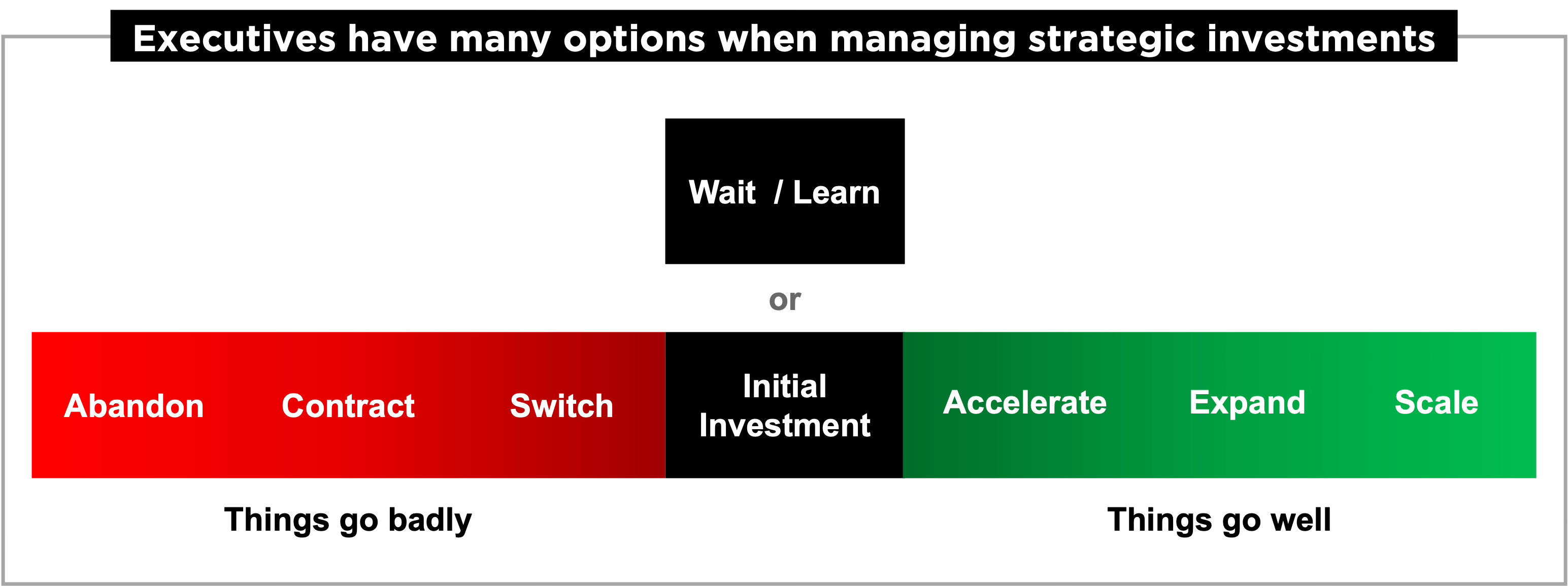
Once an initiative is launched and an initial investment is made, things can go well or badly. If things go well, executives can accelerate the initiative or expand its scope or scale (while providing the required additional investment). If things go badly, executives can switch the company’s approach as it gains knowledge and experience, reduce the size or scope of the initiative, or abandon it.
While this may seem obvious, it may not be obvious that valuation approaches such as NPV ignore managerial flexibility. NPV and similar valuation approaches assume:
investment decisions must be made immediately and
whatever execution plan is modeled initially will be followed without modification for the duration of the forecast horizon.
Anyone with any business experience knows both assumptions are invalid. Because these invalid assumptions are embedded in the methodologies, they result in erroneous valuations and poor investment decisions.
Consider a company deciding whether to enter an emerging product market (Figure 4). The company is reasonably certain it will cost $10M to develop and launch the product over the next year. It is uncertain about the strength of future demand for the product (for simplicity, this is the only uncertainty being modeled).
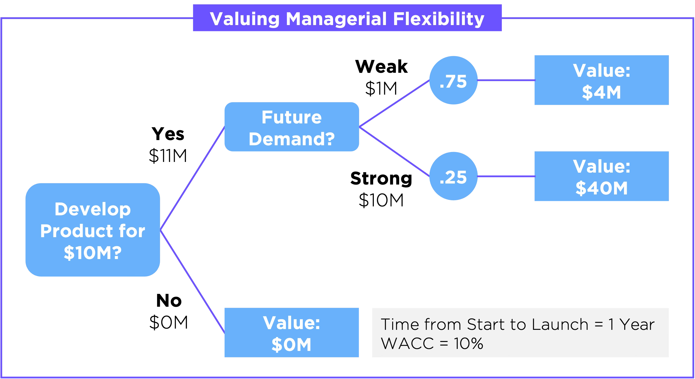
The company thinks there is a 75% chance that demand will be weak, adding only $4M in economic value (the net value of all future revenues, costs, taxes, etc. associated with the product). If demand is strong, the company expects it could add $40M in economic value.
Readers who don’t like math or Finance can skip the rest of this section, which demonstrates that using NPV leads to the wrong decision because it ignores managerial flexibility.
Since there is a 75% chance of making $4M and a 25% chance of making $40M, the expected value of the investment is (0.75 x $4M) + (0.25 x $40M) = $1M + $10M = $11M.
Since this value will not be earned until a year from now (due to the delay required to develop/launch the product), the future value ($11M) must be discounted to determine its present value (again, because money received in the future is worth less than money received today).
The discount rate for this money is the company’s Weighted Average Cost of Capital (WACC), which is 10%.
Table 2 depicts the NPV calculation for this prospective investment.
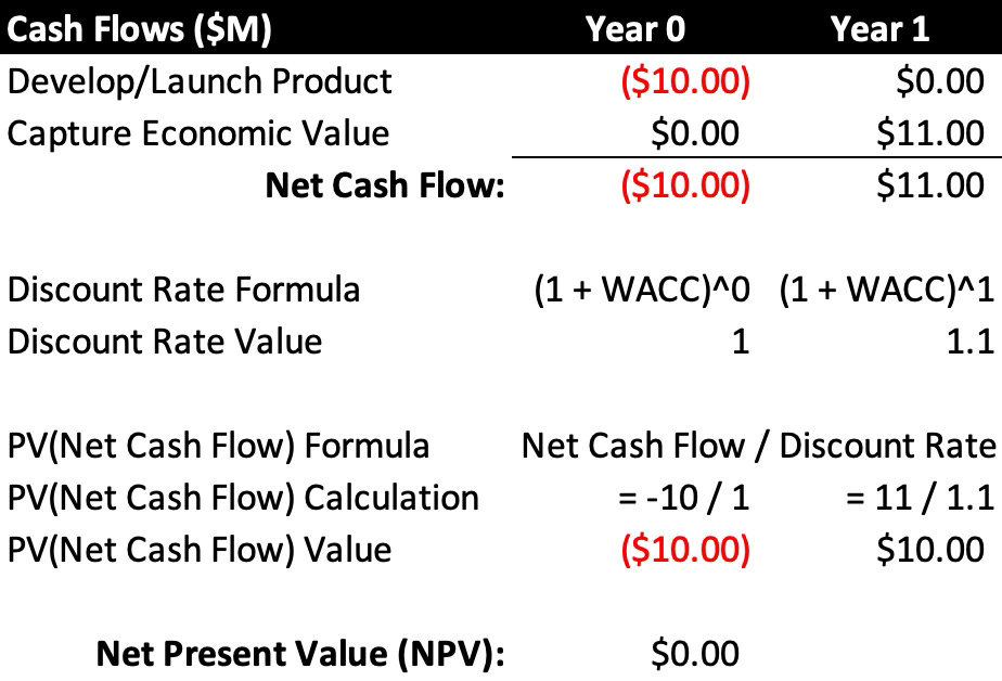
In Year 0, the company will spend $10M to develop and launch the product. In future years (represented by a single value in Year 1 to simplify things), it will capture $11M in economic value.
The discounted value of the net cash flows in Year 0 is -$10M. The discounted value of the net cash flows in Year 1 is $10M. Thus, the Net Present Value of the cash flows (again, the value on the day the decision is made) is -$10M + $10M = $0.
Standard investment guidelines state that decision-makers should reject a project with an NPV less than or equal to zero. Thus, if the company uses NPV as its decision-support tool, it will not enter this emerging product market. End of story.
Table 3 depicts a somewhat more complicated NPV calculation for this prospective investment, modeling the flexibility ignored in Table 2. (This is not an ROV calculation, but it captures the value of delaying an investment decision until a key uncertainty is reduced or resolved.)
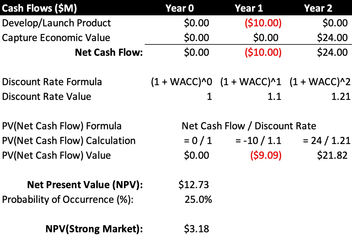
The company has the option to wait one year and enter the emerging product market only if demand is strong. In this case, the $10M expenditure to develop/launch the product will occur in Year 1, and the economic value will be captured in Year 2. However, the value the company captures will be reduced by 40% due to its delayed market entry.
Because the uncertainty involving the demand would be resolved before the investment is made, the company will capture $24M ($40M x [1 - 40%]) in economic value. However, there is only a 25% chance this will happen, so the NPV must be reduced to reflect the probability of this outcome.
As you can see, the NPV is positive, so the company should defer its investment and monitor market developments rather than abandon the idea, as it did in the first case.
Again, it may be obvious that the company could simply wait and see what happens. However, the traditional NPV approach could result in the company committing resources to other initiatives and failing to monitor developments in this emerging market. In such a case, it would be caught off-guard and unprepared or unable to make this commitment in the future.
In addition to delaying the decision, the company has the option of launching one or more strategic experiments to learn more about this emerging market and how best to meet emerging demand (Table 4).
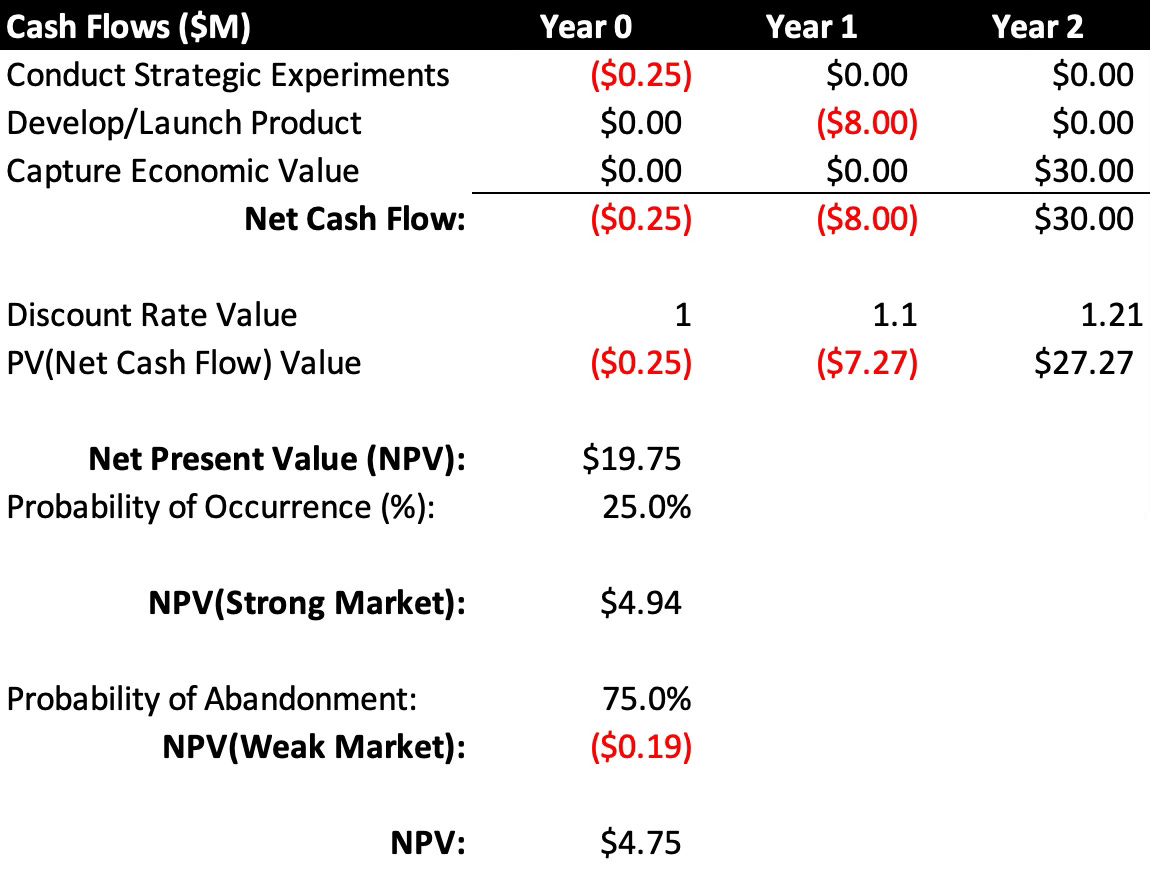
In this case, the company spends $250K in Year 0 on a set of strategic experiments. What it learns about market needs and how to meet them enables the company to reduce planned product development expenditures by 20% and reduce the loss of value from its late market entry from 40% to 25%.
There is a 25% chance demand will be strong, so the NPV associated with this outcome must be reduced to reflect this probability. There is a 75% chance demand will be weak. In this case, the $250K spent on experimentation will be lost, and the project will be abandoned. The NPV for the project is adjusted to reflect the probability of abandonment.
As you can see, the highest NPV of the three cases results from conducting strategic experiments, so company decision-makers should choose this course of action.
You may be thinking that NPV can be used to capture managerial flexibility since Case 2 and Case 3 demonstrate this. Many companies pair their valuation methodology with decision trees and other constructs to model flexibility and uncertainty more accurately. Such approaches get complicated very quickly and are still limited to a small subset of discrete values.
This approach is plausible only because I limited the uncertainty to market demand. In a real-life situation with the same structure, there would be uncertainty regarding:
development costs
the development timeline
the probability of strong market demand
the value that could be captured if demand is weak
the value that could be captured if demand is strong
the loss of value due to delayed market entry
More complex problem structures would have many more uncertainties, making modeling this way very difficult to construct and maintain. Even if it were possible, there would still be only two or three discrete values at each node in the tree rather than the entire range of values that ROV can support (via Monte Carlo Simulation).
ROV is better equipped than hybrid approaches to model the uncertainty and managerial flexibility inherent in prospective investment decisions.
Real Option Valuation
Real Options are derived from the Black-Scholes options pricing model developed in 1973. Real Option Valuation resulted from the insight that the same principles used to value market-traded options could be applied to business decisions where uncertainty and timing play crucial roles.
The math underlying ROV is much more complicated than the math underlying approaches such as NPV. Building ROV models also takes more time and effort, so executives shy away from using them. By rejecting them, executives fail to account for many uncertainties and inadvertently accept the related risks, as demonstrated in Case 1 above.
Real Options should be added to the strategic management toolkit, but they should be used only in appropriate situations. They are most appropriate when companies face:
A high degree of economic risk or
Medium to high strategic uncertainty, such as R&D projects, new product/service developments, and new market entries, or when the business environment is characterized by rapid technological change, high market volatility, or rapidly evolving competitive and regulatory landscapes.
The equation used to calculate ROV is similar in structure to that used to calculate NPV.
NPV = PV(Cash Inflows) – PV(Cash Outflows)
ROV = (PV(Cash Inflows) x Adjustment Factors) – (PV(Cash Outflows) x Adjustment Factors)
Cash Inflows are adjusted to reflect any loss of value from not making the investment (such as the expected value lost for late market entry) and to reflect the likelihood of a positive outcome based on current circumstances.
Cash Outflows are adjusted to reflect the risk-free interest that can be earned on the money not used for the investment and for the likelihood that the investment will be made in the future.
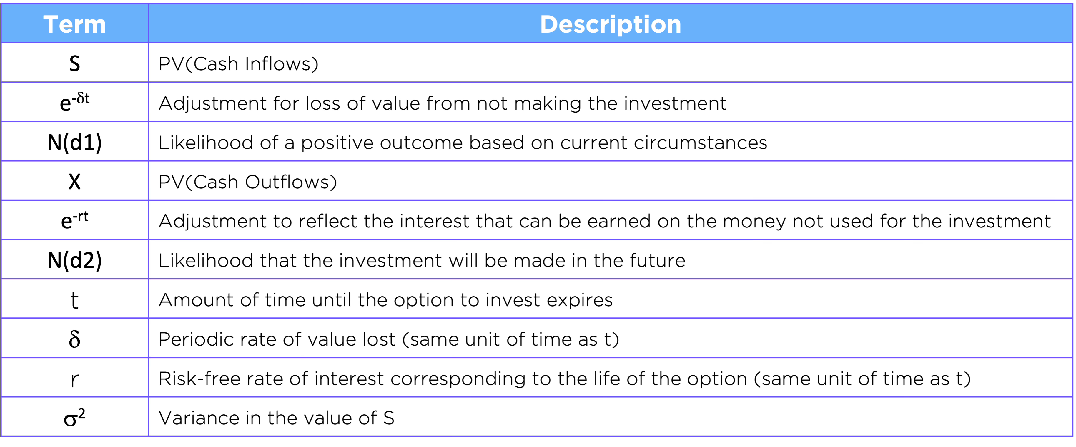
The actual equation is shown below for completeness. Table 5 describes all terms.
ROV = Se-𝞭t N(d1) – Xe-rt N(d2)
d1 = [ln(S/X) + (r - 𝞭 + 𝛔2/2)t]/(𝛔√t)
d2 = d1 - 𝛔√t
Using the values calculated in Case 3 above (Table 4) and plugging them into the ROV equation results in an ROV of $14.07M (Table 6).
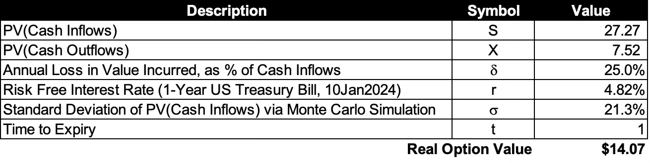
The value calculated using ROV is much higher than the combination of the decision tree and NPV used in Case 3. Much of the additional value is driven by the variance in the cash flows and the interest earned, neither of which is accounted for in Case 3.
For a limited but more straightforward way to calculate ROV, I recommend Investment Opportunities as Real Options: Getting Started on the Numbers by Timothy Luehrman, Harvard Business Review, July-August 1998.
Despite how complicated and intimidating these equations may look, they can be calculated fairly easily using a spreadsheet (as shown in Table 6). Please note that the valuations produced are less important than the relative values among a set of strategic options.
Executives should focus on managing the drivers of value and uncertainty rather than the equation, and on adopting a Real Options mindset to improve strategic decision-making and strategic agility. For example, in Case 3 above, strategic experiments were run that reduced development costs (X, the PV of cash outflows), reduced the value lost by delayed market entry (𝞭), and kept open an option for entering an emerging product market that would have been abandoned using NPV.
In general, executives can increase the value of company options by:
Increasing PV(Cash Inflows) (S)
Reducing PV(Cash Outflows) (X)
Increasing the uncertainty of cash inflows (𝛔) (Since there is limited downside due to the option, the more variable the cash flows, the more likely they will increase above the cost of the option, creating higher profits when the option is exercised.)
Increasing the duration of the option (t)
Reducing the value lost while waiting to exercise the option (𝞭)
Although not under managerial control, option values increase as risk-free interest rates (r) increase because the company can earn more interest on the money it has not invested yet.
If you would like more specific advice on how to manage the ROV levers in ways that increase value, please ask via the comments section or contact me directly.